One of the code examples that Colab provides handles recording of an image via a webcam. The code writes a webcam frame to an image file and displays it. However, it does not directly handle life streaming of the webcam feed.
In short, it uses the same interface as the example to pass the frame via javascript from the browser to the Colab Runtime. Therefore, the frame data is converted to a Data URL, i.e., compressed as a jpeg and base64 encoded.
The python backend decodes the image string and decompresses the jpeg data.
As I wanted to visualize the data as well, passing data from python to the javascript caller is also demonstrated.
A word of caution: While the approach does work, the performance is clearly not good and the number of frames you are able to process per second is very limited.
I’ve been searching my files for a while to find the dataset of a replication of Yarbus’ famous experiment. Seems like the webpage of Ali Borji ( http://ilab.usc.edu/borji/Resources.html ) mentioned in the manuscript does not link to the data anymore. However, it’s still available via the direct download link at http://ilab.usc.edu/borji/Yarbus.zip
Ball B-splines are used to model tube-like 3D surfaces or volumes. You can imagine them as a rubber hull over a sequence of marbles of variable diameter. The concept is almost identical to that of normal B-splines: We fit a polynomial to small segments of the complete curve. By combining multiple piecewise polynimials we can constuct an arbitrary shape. Key to this procedure is that the stitching between polynomials is smooth, meaning that we can place one polynomial at the end of the previous one without any visible border, offset or spontaneous direction change.
The splines are defined by so-called control points, i.e., the points that we fit the polynomials against. Usually, these points will not be located on the final polynomial, but only approximated by them (a property that is non-advantageous in some situations). Smoothness between neighboring polynomials is achieved by the use of two weighting functions that ramp up (down) from 0 to 1 (and vice versa) as we get closer to an edge point of the segment.
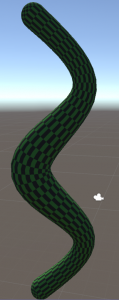
Ball B-spline representation of a primitive snake. A tasty rabbit meal is contained in the midst of its body (thicker area).
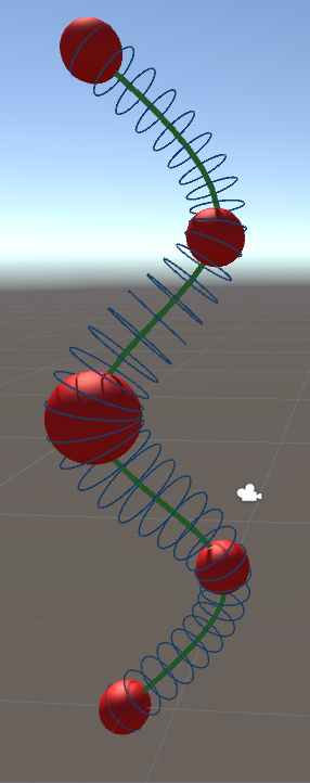
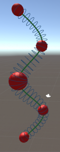
Skeleton of the snake with key-spheres shown in red. The green line indicates the center position spline, the blue circles the radius at the respective position.
For example, imagine how a snake eats and digests a rabbit. The victim’s body would slowly traverse from the snake’s head towards its tail. The resulting bulb in the snake’s body shape would slowly decrease during the prey’s travel through the digestive tract. Transferred to Ball B-Splines we could create a snake by defining some spheres, one for the head and a smaller one for the tail (and some along the sinus curve to make it snaky [ideally, one would sample at the extrema of the sinus function so that the polynomial is in shape even for only few keypoints).
We can then model the tasty meal by an additional sphere somewhere between the snake’s head and its tail. The rabbit’s transition through the snake’s gut would simply be a movement of this sphere from head to tail (along the green center line) and a decrease in diameter simulates its digestion. Enjoy your meal.
To highlight the elegance of the approach: In order to simulate how the snake is moving around, one would only need to move the few keypoints. The remainder of the mesh would move along with them accordingly.
In the following posts I will go into more detail on the steps required to create such a Ball B-spline mesh. All sourcecode is availale at my github.
This step is part of an approach to procedural tree modelling. Ao, Xuefeng, Zhongke Wu, and Mingquan Zhou proposed the Ball B-spline architecture to represent the tree skeleton: “Real time animation of trees based on BBSC in computer games.” International Journal of Computer Games Technology 2009 (2009): 5.
A general introduction to Ball-B-splines (without many directly useful formulas, but more of an overview) is provided by Wu, Zhongke, Hock Soon Seah, and Mingquan Zhou. “Skeleton based parametric solid models: Ball B-Spline curves.” Computer-Aided Design and Computer Graphics, 2007 10th IEEE International Conference on. IEEE, 2007.
This post will be about the first step in both Guiding Vector Tree and Space Colonialization algorithms: Poisson sampling. Both procedurally generate a tree structure by joining either randomly sampled points together or by summing over a randomly ampled set of attraction points. But the straight-forward approach
while (nGeneratedSamples < nRequestedSampled)
    new Sample(Random.value, Random.value, Random.value)
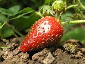
Distribution of strawberry nuts over its surface. Image by kai-Martin Knaak [CC-BY-SA-3.0 (http://creativecommons.org/licenses/by-sa/3.0/)], via Wikimedia Commonhas some flaws. The most important one is the distribution that we draw the random number from. A uniform distribution (i.e., rolling a dice where each face has the same probability to be chosen) does often not correspond to what we humans perceive as randomness – because processes we encounter in nature are often everything but randomized, even though we call them so. For example, the distribution of nuts over the surface area of a strawberry might look relatively random at first glance. However, we will find no two nuts positioned significantly closer to each other than all the others. In the following we will look at two methods to generate samples in a “strawberry nut way”.
Fast Poisson disk sampling
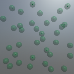
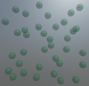
Poisson Disk sampling in 3D with the disks shown as semi-transparent hulls around the darker samples.
There is a nice and general implementation for the 2D case available at [2] with some hints for extending it to 3D. Here is a quick overview what happens within that algorithm:
The approach by Bridson [3] starts with a seed point P1 and repeatedly “throws a dart” (Poisson-speech for choosing a random point) from the neighborhood of P1. This point P1 is chosen so that a minimum distance of r_min and a maximum distance of r_max towards P1 is guaranteed. Next, we need to check whether P1 violates the neighborhood criteria (= is too close to) any other of our previously sampled points. If so, throw another dart. If not, P1 is a good sample and we take it. In case we threw 30 darts in the neighborhood of P0 and did not find any free position, we consider that neighborhood filled and proceed with sampling around P1. Thereby, the sampled area gradually grows outwards with each dart thrown and accepted. That means that the sampled area gradually grows outwards and also implies that the sampling is only complete, if there is no other location to grow to left.
Because of this growth process and the heuristic 30 darts thrown it is possible that some locations remain undersampled. There might even be holes in your sample volume that still require to be closed. Most importantly, you are required to perform the algorithm until the 30-darts criterium was completed for all your samples. Before the completion your sampling is probably incomplete and contans relevant holes. The original publication of this approach [3] proposes a reasonably fast way of sampling in arbitrary dimensions, not just in two as shown in the above mentioned blog.
But there are some caveats that I want to point at. As an approximation, the authors propose throwing 30 darts to determine whether the neighborhood of a sample is already full – if none of them hits an unoccupied spot, there probably is none (thus we get an approximation of the desired distribution, but a rather good one [4]). As growing trees is not exactly a high precision thing, a reasonable approximation is fine for our purpose and the speed gain (Ο(n) versus Ο(n log(n)) for accurate sampling [4]) is probably worth it. I’ll dive into the code for the 3D case in a later post.
Grid jitter
Grid jitter with a relatively small jitter range. The original (non-jittered) sample location is contained within the semi-transparent hull sphere.
That’s because sometimes you get a bit smarter just a moment too late, for example after having implemented the above algorithm. And then you recodnize that you would be much better off with a much simpler solution. Specifically, when you are being asked to create a Yao8 graph of the generated random samples. Generating such a tree involves finding the nearest neighbor for each sample towards a certain direction. Sure, that is possible (you can use Delaunay triangulation and geenerate an Uruquhard graph from that, for example). But turns out it is algorithmically more complex than one would expect (at least when performance times matter). Thesimple brute-force solution, won’t perform well on >10.000 samples – which we will require for nice looking trees.
So for the promised, much simpler solution. It should not remain unmentioned that the other people who proposed the approach described above were aware of this simple solution but did not find the results satisfying (so it’s just me being not smart enough at the right time and having to go the extra way).
You basically populate a 3D Grid with a sample at each corner of the grid. Then you jitter these points. Simple as that. And you get a decent approximate of the neighborhood graph for absolutely free (as long as we do not jitter too much so that the graph gets messed up).
It is even possible to implement the minimum-distance criteria from above as we know about the original distance between samples and the magnitude of the jitter. Sadly, the sampling is not as nice as the disk sampling method above (just think of moving two points towards each other along the grid versus diagonally. The more in distance you need to bring them together (or to a minimum distance towards each other) diagonally (Pythagoras) is one of the reasons for that. But we are trying to produce trees here. Good Enough (plus we can do that really fast, compared to throwing lots and lots of darts).
Outlook: Next post will either discuss interesting code segments for both sampling routines or Ball B-Spline curves.
[1] Xu, L., & Mould, D. (2015, October). Procedural tree modeling with guiding vectors. In Computer Graphics Forum (Vol. 34, No. 7, pp. 47-56).
[2] http://devmag.org.za/2009/05/03/poisson-disk-sampling/
[3] Bridson, R. (2007, August). Fast Poisson disk sampling in arbitrary dimensions. In SIGGRAPH sketches (p. 22).
[4] Gamito, M. N., & Maddock, S. C. (2009). Accurate multidimensional Poisson-disk sampling. ACM Transactions on Graphics (TOG), 29(1), 8.
Recently I stumbled across the Procedural World Blog (https://procworld.blogspot.de/). It has a nice post on how to generate trees algorithmically. They use the so-called Space Colonialization algorithm [1]. Basically, a large number of attraction-points is chosen randomly within the volume of the soon-to-be tree crown and each of these points excerts an influence on the sequentially growing branches. That post is from 2010 and there has been considerable progress. Just a quick glance into literature:
Space Colonialization is actually based on a publication on leaf ventilation patterns (the branching structures within a leaf) [2]. The authors found that what works for leafes only needs some minor adjustments to be applicable to whole trees [1]. Copy, transform, combine – that’s how nature works after all.
Guiding Vector Trees are created by choosing shortest paths between randomly sampled points within a volume. To avoid a straight line from the stem towards the tip of the branch, path weights are calculated by the distance towards the direction of a guiding vector. That is a vector that changes gradually based upon the vector of the parent node [3]. The authors worked towards this method in two prior publications that propose very similar algorithms [4,5] and might be helpful to understand some of the details.
Procedural Branch Graph is a method created for fast real-time creation of trees within a virtual reality (yeah, that’s just to make it sound more fancy. You could of course use any of the above trees, if you sample a low poly version). But they propose some useful hints on how to process the 3D mesh structure of the tree for performance [6].
Furthermore there are some interesting approaches that start with a complete tree model:
Pirk et al. animate a naturalistic growth process [7].
Again Pirk et al. show how to transform a tree skeleton so that it responds to obstacles and lightning in its proximity [8].
Ao et al. choose a clever representation of the tree structure, called Ball B-Spline Curves, that allows for a cheaper calculation of motion [9]. Moving tree meshes – well that’s cool.
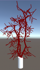
Personally, I find the Guiding Vector Tree approach promising. The rendered images provided in the paper show some convincing examples of really beautiful, realistic-looking trees. In the following posts I’ll explain some of the details of implementing such an approach in C# and Unity.
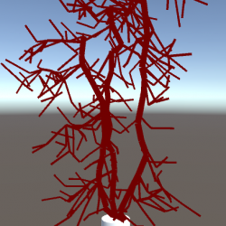
A tree structure generated by the Guiding Vector Tree approach. Not exactly a beauty yet – but single line rendering seldomly is.
Sources
[1] Runions, Adam, Brendan Lane, and Przemyslaw Prusinkiewicz. “Modeling Trees with a Space Colonization Algorithm.” NPH 7 (2007): 63-70.
[2] Runions, Adam, et al. “Modeling and visualization of leaf venation patterns.” ACM Transactions on Graphics (TOG) 24.3 (2005): 702-711.
[3] Xu, L., & Mould, D. (2015, October). Procedural tree modeling with guiding vectors. In Computer Graphics Forum (Vol. 34, No. 7, pp. 47-56).
[4] Xu, Ling, and David Mould. “Synthetic tree models from iterated discrete graphs.” Proceedings of Graphics Interface 2012. Canadian Information Processing Society, 2012.
[5] Xu, Ling, and David Mould. “A procedural method for irregular tree models.” Computers & Graphics 36.8 (2012): 1036-1047.
[6] Kim, Jinmo. “Modeling and Optimization of a Tree Based on Virtual Reality for Immersive Virtual Landscape Generation.” Symmetry 8.9 (2016): 93.
[7] Pirk, Sören, et al. “Capturing and animating the morphogenesis of polygonal tree models.” ACM Transactions on Graphics (TOG) 31.6 (2012): 169.
[8] Pirk, Sören, et al. “Plastic trees: interactive self-adapting botanical tree models.” ACM Transactions on Graphics 31.4 (2012): 1-10.
[9] Ao, Xuefeng, Zhongke Wu, and Mingquan Zhou. “Real time animation of trees based on BBSC in computer games.” International Journal of Computer Games Technology 2009 (2009): 5.
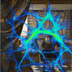
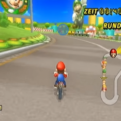
Ever wondered how your eyes perform while playing a videogame? Turns out they might be quite important for you winning the game. Actually, so important that one can even distinguish whether you are a winner based solely on the movement of your eyes! And here is, what eye-tracking whilst gaming looks like:
The small blue dots are called fixations, i.e. the spots where the eye rests at (even if it does so only shortly). During a fixation we actually perceive visual information. Fixations are interconnected by saccades, very very fast movements of the eye. In fact, they are so super-fast that our brain suppresses visual perception while we perform them. Try it with a mirror – you won’t be able to see your eyes moving when you look from one spot to the other.
Eye-tracking data comparison
So when you do an eye-tracking experiment, the result is just a list of fixation locations (and durations) and the saccades in-between. May look fancy on youtube, but doesn’t actually tell you anything meaningful most of the time. What you need to do is calculate some key metrics (such as the average time spent looking at the same location before shifting gaze; or the gaze density at certain game objects).
Comparing eye movement sequences to each other as a whole (without the restriction to one specific key metric) is non-trivial (and I will likely cover this in a future post, as this is my PhD topic 😉 ). But if we do so, turns out that we can separate good players from novices quite well (Figure 1). It’s not just reactions that we train and getting to know the game better – but also a training effect in the patterns of how we need to move our eyes, that make a good player.
Figure 1: The percentage of scanpaths classified correctly as either fast or slow drivers is shown on the diagonal. Off-diagonal elements (left top and bottom right) are misclassifications.
T. C. Kübler, C. Rothe, U. Schiefer, W. Rosenstiel, E. Kasneci (2016): SubsMatch 2.0: Scanpath comparison and classification based on subsequence frequencies. Behavior Research Methods:1-17
Saliency is a measure of how strong elements stand out from their surrounding. Highly salient objects are likely to attract an observer’s attention. These regions are usually viewed during the first fixations, within very few seconds or even milliseconds. Are you interested in what people will look at in your image/website/advertisement?
Give it a try:
Original image
or use your own image:
Processing progress:
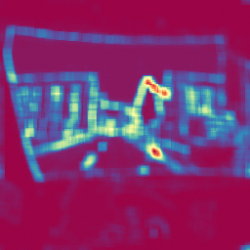
Saliency map
Residual filter length:
Postprocess smoothing:
There are several ways to computationally calculate saliency and all of them somehow highlight large color and intensity contrasts in the image. Depending on which method you prefer, the calculation is inspired by the human retina and visual processing pipeline, or just a plain piece of math (less physilogically meaningful but not necessarily less accurate when it comes to predicting observer’s gaze).
While image based saliency is an indicator of where attention will be directed to, it is entirely a bottom-up approach. That means that no knowledge of the viewer is included in the model. However, we humans have developed clever viewing strategies to tackle certain tasks, such as viewing web pages. To get a depper understanding of where we actually look at – and which cognitive associations are involved – there is currently no way around an eye-tracking study.
All data processing in this application is client-sided, meaning that neither your image nor the generated saliency map is transferred to any computer but yours.
Some remarks: The above saliency map computation works on gray-scale images. Even if you provide a color image, the implementation will convert it to grayscale. Theoretically, one could (and should) combine multiple saliency maps computed on different color spaces to get better results.
Hou, Xiaodi and Zhang, Liqing (2007): Saliency detection: A spectral residual approach. 2007 IEEE Conference on Computer Vision and Pattern Recognition:1-8
Map colors based on www.ColorBrewer.org, by Cynthia A. Brewer, Penn State.
Fourier Transform in Javascript by Anthony Liu.