Ball B-splines

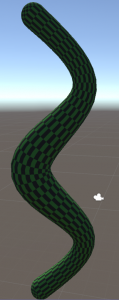
Ball B-splines are used to model tube-like 3D surfaces or volumes. You can imagine them as a rubber hull over a sequence of marbles of variable diameter. The concept is almost identical to that of normal B-splines: We fit a polynomial to small segments of the complete curve. By combining multiple piecewise polynimials we can constuct an arbitrary shape. Key to this procedure is that the stitching between polynomials is smooth, meaning that we can place one polynomial at the end of the previous one without any visible border, offset or spontaneous direction change.

The splines are defined by so-called control points, i.e., the points that we fit the polynomials against. Usually, these points will not be located on the final polynomial, but only approximated by them (a property that is non-advantageous in some situations). Smoothness between neighboring polynomials is achieved by the use of two weighting functions that ramp up (down) from 0 to 1 (and vice versa) as we get closer to an edge point of the segment.

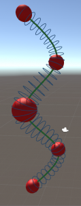
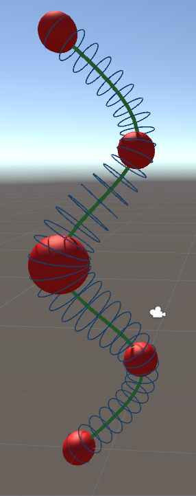
For example, imagine how a snake eats and digests a rabbit. The victim’s body would slowly traverse from the snake’s head towards its tail. The resulting bulb in the snake’s body shape would slowly decrease during the prey’s travel through the digestive tract. Transferred to Ball B-Splines we could create a snake by defining some spheres, one for the head and a smaller one for the tail (and some along the sinus curve to make it snaky [ideally, one would sample at the extrema of the sinus function so that the polynomial is in shape even for only few keypoints).

We can then model the tasty meal by an additional sphere somewhere between the snake’s head and its tail. The rabbit’s transition through the snake’s gut would simply be a movement of this sphere from head to tail (along the green center line) and a decrease in diameter simulates its digestion. Enjoy your meal.

To highlight the elegance of the approach: In order to simulate how the snake is moving around, one would only need to move the few keypoints. The remainder of the mesh would move along with them accordingly.

In the following posts I will go into more detail on the steps required to create such a Ball B-spline mesh. All sourcecode is availale at my github.

This step is part of an approach to procedural tree modelling. Ao, Xuefeng, Zhongke Wu, and Mingquan Zhou proposed the Ball B-spline architecture to represent the tree skeleton: “Real time animation of trees based on BBSC in computer games.” International Journal of Computer Games Technology 2009 (2009): 5.

A general introduction to Ball-B-splines (without many directly useful formulas, but more of an overview) is provided by Wu, Zhongke, Hock Soon Seah, and Mingquan Zhou. “Skeleton based parametric solid models: Ball B-Spline curves.” Computer-Aided Design and Computer Graphics, 2007 10th IEEE International Conference on. IEEE, 2007.