Procedural Tree – Poisson Disk Sampling in 3D (C#)

This post will be about the first step in both Guiding Vector Tree and Space Colonialization algorithms: Poisson sampling. Both procedurally generate a tree structure by joining either randomly sampled points together or by summing over a randomly ampled set of attraction points. But the straight-forward approach

while (nGeneratedSamples < nRequestedSampled) 
    new Sample(Random.value, Random.value, Random.value)

has some flaws. The most important one is the distribution that we draw the random number from. A uniform distribution (i.e., rolling a dice where each face has the same probability to be chosen) does often not correspond to what we humans perceive as randomness – because processes we encounter in nature are often everything but randomized, even though we call them so. For example, the distribution of nuts over the surface area of a strawberry might look relatively random at first glance. However, we will find no two nuts positioned significantly closer to each other than all the others. In the following we will look at two methods to generate samples in a “strawberry nut way”.

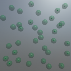
 Fast Poisson disk sampling

There is a nice and general implementation for the 2D case available at [2] with some hints for extending it to 3D. Here is a quick overview what happens within that algorithm:

The approach by Bridson [3] starts with a seed point P1 and repeatedly “throws a dart” (Poisson-speech for choosing a random point) from the neighborhood of P1. This point P1 is chosen so that a minimum distance of r_min and a maximum distance of r_max towards P1 is guaranteed. Next, we need to check whether P1 violates the neighborhood criteria (= is too close to) any other of our previously sampled points. If so, throw another dart. If not, P1 is a good sample and we take it. In case we threw 30 darts in the neighborhood of P0 and did not find any free position, we consider that neighborhood filled and proceed with sampling around P1. Thereby, the sampled area gradually grows outwards with each dart thrown and accepted. That means that the sampled area gradually grows outwards and also implies that the sampling is only complete, if there is no other location to grow to left.

Because of this growth process and the heuristic 30 darts thrown it is possible that some locations remain undersampled. There might even be holes in your sample volume that still require to be closed. Most importantly, you are required to perform the algorithm until the 30-darts criterium was completed for all your samples. Before the completion your sampling is probably incomplete and contans relevant holes. The original publication of this approach [3] proposes a reasonably fast way of sampling in arbitrary dimensions, not just in two as shown in the above mentioned blog.

But there are some caveats that I want to point at. As an approximation, the authors propose throwing 30 darts to determine whether the neighborhood of a sample is already full – if none of them hits an unoccupied spot, there probably  is none (thus we get an approximation of the desired distribution, but a rather good one [4]). As growing trees is not exactly a high precision thing, a reasonable approximation is fine for our purpose and the speed gain (Ο(n) versus Ο(n log(n)) for accurate sampling [4]) is probably worth it. I’ll dive into the code for the 3D case in a later post.

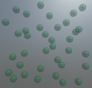
Grid jitter

That’s because sometimes you get a bit smarter just a moment too late, for example after having implemented the above algorithm. And then you recodnize that you would be much better off with a much simpler solution. Specifically, when you are being asked to create a Yao8 graph of the generated random samples. Generating such a tree involves finding the nearest neighbor for each sample towards a certain direction. Sure, that is possible (you can use Delaunay triangulation and geenerate an Uruquhard graph from that, for example). But turns out it is algorithmically more complex than one would expect (at least when performance times matter). Thesimple brute-force solution, won’t perform well on >10.000 samples – which we will require for nice looking trees.

So for the promised, much simpler solution. It should not remain unmentioned that the other people who proposed the approach described above were aware of this simple solution but did not find the results satisfying (so it’s just me being not smart enough at the right time and having to go the extra way).

You basically populate a 3D Grid with a sample at each corner of the grid. Then you jitter these points. Simple as that. And you get a decent approximate of the neighborhood graph for absolutely free (as long as we do not jitter too much so that the graph gets messed up).

It is even possible to implement the minimum-distance criteria from above as we know about the original distance between samples and the magnitude of the jitter. Sadly, the sampling is not as nice as the disk sampling method above (just think of moving two points towards each other along the grid versus diagonally. The more in distance you need to bring them together (or to a minimum distance towards each other) diagonally (Pythagoras) is one of the reasons for that. But we are trying to produce trees here. Good Enough (plus we can do that really fast,  compared to throwing lots and lots of darts).

Outlook: Next post will either discuss interesting code segments for both sampling routines or Ball B-Spline curves.

 

PS: github of the Unity source code

Sources

[1] Xu, L., & Mould, D. (2015, October). Procedural tree modeling with guiding vectors. In Computer Graphics Forum (Vol. 34, No. 7, pp. 47-56).
[2] http://devmag.org.za/2009/05/03/poisson-disk-sampling/
[3] Bridson, R. (2007, August). Fast Poisson disk sampling in arbitrary dimensions. In SIGGRAPH sketches (p. 22).
[4] Gamito, M. N., & Maddock, S. C. (2009). Accurate multidimensional Poisson-disk sampling. ACM Transactions on Graphics (TOG), 29(1), 8.